This website contains information regarding the paper Input-gradient space particle inference for neural network ensembles.

TL;DR: We introduce First-order Repulsive Deep ensembles (FoRDEs), a method that trains an ensemble of neural networks diverse with respect to their input gradients.

Please cite our work if you find it useful:

@inproceedings{trinh2024inputgradient,
    title={Input-gradient space particle inference for neural network ensembles},
    author={Trung Trinh and Markus Heinonen and Luigi Acerbi and Samuel Kaski},
    booktitle={The Twelfth International Conference on Learning Representations},
    year={2024},
    url={https://openreview.net/forum?id=nLWiR5P3wr}
}

Repulsive deep ensembles (RDEs) [1]

Description: Train an ensemble \(\{\boldsymbol{\theta}_i\}_{i=1}^M\) using Wasserstein gradient descent [2], which employs a kernelized repulsion term to diversify the particles to cover the Bayes posterior \(p(\boldsymbol{\theta} | \mathcal{D}) \).

• The driving force directs the particles towards high density regions of the posterior
• The repulsion force pushes the particles away from each other to enforce diversity.

Problem: It is unclear how to define the repulsion term for neural networks:

• Weight-space repulsion is ineffective due to overparameterization and weight symmetries.
• Function-space repulsion often results in underfitting due to diversifying the outputs on training data.

First-order Repulsive deep ensembles (FoRDEs)

Possible advantages:

• Each member is guaranteed to represent a different function;
• The issues of weight- and function-space repulsion are avoided;
• Each member is encouraged to learn different features, which can improve robustness.

Defining the input-gradient kernel \(k\)

Given a base kernel \(\kappa\), we define the kernel in the input-gradient space for a minibatch of training samples \(\mathcal{B}=\{(\mathbf{x}_b, y_b\}_{b=1}^B\) as follows:

We choose the RBF kernel on a unit sphere as the base kernel \(\kappa\):

Tuning the lengthscale \(\boldsymbol{\Sigma}\)

Each lengthscale is inversely proportional to the strength of the repulsion force in the corresponding input dimension:

Proposition: One should apply strong forces in high-variance dimensions (more in-between uncertainty) and weak forces in low-variance dimensions (less in-between uncertainty).

• Use PCA to get the eigenvalues and eigenvectors of the training data: \(\{ {\color{red}\mathbf{u}_d},{\color[RGB]{68,114,196}\lambda_d}\}_{d=1}^D\)
• Define the base kernel:
  • \( {\color{red}\mathbf{U}} = \begin{bmatrix} {\color{red}\mathbf{u}_1} & {\color{red}\mathbf{u}_2} & \cdots & {\color{red}\mathbf{u}_D} \end{bmatrix} \) is a matrix containing the eigenvectors as columns.
  • \( {\color[RGB]{68,114,196}\boldsymbol{\Sigma}^{-1}_{\alpha}} = (1-\alpha)\mathbf{I} + \alpha {\color[RGB]{68,114,196}\boldsymbol{\Lambda} } \) where \( \color[RGB]{68,114,196}\boldsymbol{\Lambda} \) is a diagonal matrix containing the eigenvalues.

Illustrative experiments

For a 1D regression task (above) and a 2D classification task (below), FoRDEs capture higher uncertainty than baselines in all regions outside of the training data. For the 2D classification task, we visualize the entropy of the predictive posteriors.

Lengthscale tuning experiments

• Blue lines show accuracies of FoRDEs, while dotted orange lines show accuracies of Deep ensembles for comparison.
• When moving from the identity lengthscale \(\mathbf{I}\) to the PCA lengthscale \(\color[RGB]{68,114,196}\boldsymbol{\Lambda}\):
  • FoRDEs exhibit small performance degradations on clean images of CIFAR-100;
  • while becomes more robust against the natural corruptions of CIFAR-100-C.

Benchmark comparison

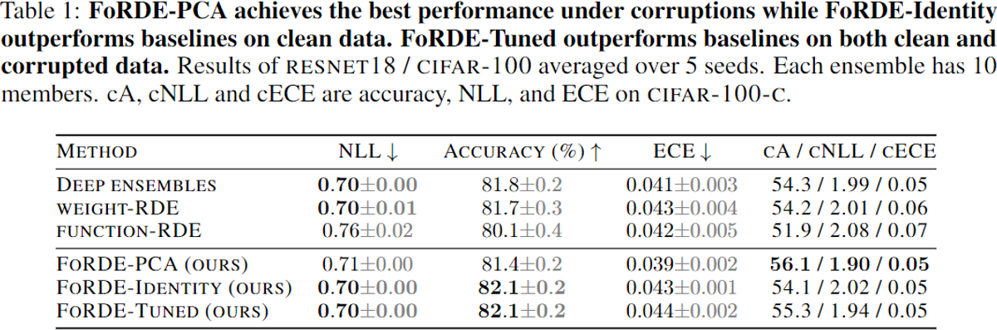
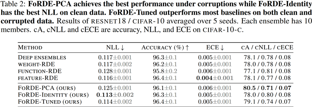
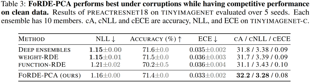
Main takeaways

1. Input-gradient-space repulsion can perform better than weight- and function-space repulsion.
2. Better corruption robustness can be achieved by configuring the repulsion kernel using the eigen-decomposition of the training data.

References

[1] F. D’Angelo and V. Fortuin, “Repulsive deep ensembles are Bayesian,” Advances in Neural Information Processing Systems, vol. 34, pp. 3451–3465, 2021.

[2] C. Liu, J. Zhuo, P. Cheng, R. Zhang, and J. Zhu, “Understanding and Accelerating Particle-Based Variational Inference,” in International Conference on Machine Learning, 2019.